Cheatsheet – Selecting Graphs for Statistical Analysis

One of the first steps with any statistical analysis, whether for hypothesis testing or predictive analytics or even a Kaggle competition, is checking the relationship between different variables. Checking if a pattern exists.

Graphs are a fantastic and visual way of identifying such relationships.
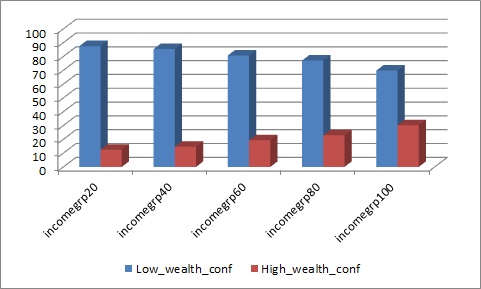
graph-matplotlib

MATPLOTLIB Graph

However, numerous readers kept getting stuck while selecting graphs for categorical variables and many friends asked if there was a standard rule for graph selection. With that in mind, please see below a cheatsheet for graphical selection for both quantitative (numeric) and categorical ( character -gender, disease type, etc.) variables.


 No.

Axis1

Axis2

Chart type

1.

Single quant

Histograms, Density plot, Box plot
2.

Single categorical

Bar chart (freq/ count), Pie chart (freq/ count/%)
2.

Categorical

Quant

Bar chart, pie chart, frequency table, line chart
3.

Quant

Quant

Scatterplot
4.

Categorical

Categorical

Stacked Column Chart, combination chart (typical bar chart with trendlines)
5.

2 categorical

Quant

Stacked or side-by-side bar charts, heat maps. Any basic graph, with Color/shape code for one of the quant variables.
6.

1 categorical

2 Quant

Stacked or side-by-side bar charts, Scatter plots. Any basic graph, with Color/shape code for one of the quant variables.
7.

3+ variables of any type

Please check if you really need so many variables in a single graph. Side-by-side graphs may be a better option, or graphs with filters (if possible based on the programming language)

These are merely guidelines and are language-agnostic, so you may choose to implement them in your choice of programming language ( R, Python, SAS, MATLAB, etc.) . However, if you prefer, code implementations in R and Python are provided in the links below:

  • Charts in R :
  • Charts in Python :
    • This link contains code and images to create stunning graphs (box plots, histograms, heatmaps, bubble charts, etc) using MATPLOTLIB library, like the one shown above.

Hope you find this cheatsheet useful! Feel free to share your thoughts and comments. Adieu!

25+ free datasets for Datascience projects

Here are top 25 websites to gather datasets to use for your data science projects in R, Python, SAS, Excel or other programming language or statistical software. Best part, these are all free, free, free! 

Cloud 1

25 Free Datasets for DataScience & BigData Projects

Government and UN/World Bank websites:

  1. US government database with 190k+ datasets –http://catalog.data.gov/dataset
  2. UK government database with 25k+ datasets – https://data.gov.uk/data/search
  3. Canada government database – http://open.canada.ca/data/en/dataset?q=education
  4. FBI crime statistics – http://1.usa.gov/1LltHEQ
  5. Center for Disease Control – http://wonder.cdc.gov/
  6. Bureau of Labor Statistics – http://www.bls.gov/data/
  7. NASA datasets – http://nssdc.gsfc.nasa.gov/
  8. World Bank Data – http://datacatalog.worldbank.org/
  9. UN database with 34 sets and 60 million records – http://data.un.org/
  10. EU commission open data – https://open-data.europa.eu/en/data/
  11. NIST – http://1.usa.gov/1JpmcNI
  12. National Center for Education Statistics – http://1.usa.gov/1mAjH0A
  13.  U.S. National Epidemiological Survey on Alcohol and Related Conditions (NESARC) – dataset from survey to determine magnitude of alcohol use and psychiatric disorders in the U.S. population.

Academic websites:

  1. Yelp academic data – https://www.yelp.com/academic_dataset
  2. Univ of California, Irvine – http://archive.ics.uci.edu/ml/datasets.html
  3. Harvard Univ: http://gis.harvard.edu/resources/data
  4. Harvard Dataverse database: http://bit.ly/1RlXNKa
  5. MIT: http://web.mit.edu/towtank/www/vivdr/datasets.html. Also, http://bit.ly/1IMJVri
  6. Univ of North Carolina, adolescent health – http://www.cpc.unc.edu/projects/addhealth/data
  7. Mars Crater Study, a global database that includes over 300,000 Mars craters 1 km or larger, provided by Wesleyan University:

 Kaggle & Datascience resources:

  1. Few of my favs from Kaggle Website
  2. Databits.io – http://databits.io/challenges/opensource . My favorites among these are :
  3. Datasets on Climate information, human genome data, Enron email information, etc – https://www.quandl.com/search?type=free
  4. Gapminder – http://www.gapminder.org/data/

Curated Lists:

  1. KDnuggets provides a great list of datasets from almost every field imaginable – space, music, books, etc. May repeat some datasets from the list above.
    http://www.kdnuggets.com/datasets/index.html
  2. An eclectic mix of datasets about gun ownership, NYPD crime rates, college student study habits and caffeine concentrations in popular beverages – https://www.reddit.com/r/datasets
  3. Data Science Central has also curated many datasets for free – http://www.datasciencecentral.com/profiles/blogs/big-data-sets-available-for-free
  4. List of open datasets from DataFloq – https://datafloq.com/public-data/?sp=6358335213372237508418

Others:

  1. MRI brain scan images and data – http://bit.ly/1kFfcke
  2. Economic, education, Health and other datasets from Quandl. Please note this site also has a premium version of other datasets – https://www.quandl.com/search?type=free
  3. Google repository of digitized books and ngram viewer – https://books.google.com/ngrams. Sample chart shown below:
  4. Database with geographical information – http://freegisdata.rtwilson.com/
  5. Loan information from Lending Club – https://www.lendingclub.com/info/download-data.action

Moderator variable with Chi-Square test

Hello All,

Today’s post is the assignment exercise for week 4 for the Coursera class on Data Visualization Tools from Wesleyan University.

The topic is as below:

Run an ANOVA, Chi-Square Test or correlation coefficient that includes a moderator.

For this round of assignments, I’m using the outlook on life dataset provided for the course, as available here. Today I am going to test the confidence to achieve secure retirement (var = W1_F4_B) based on incomegroup (INCOME, calculated from given var = PPINCIMP). The moderator variable is marital status (MARIT, computed from PPMARIT).

I am using the chi-square test for this assignment.

The hypothesis for this assignment is as follows:

  1. Ho = No relationship between INCOME and W1_F4_B.
  2. H1 = There is a significant relation between above two variables.


Procedure for Chi-Square test:

  1. INCOME variable has 5 levels :
    • 20 => income between 0 to 19,999
    • 40 => income between 20,000 to 39,999
    • 60 => income between 40,000 to 59,999
    • 80 => income between 60,000 to 99,999
    • 100 => income greater than 99,999
  2. MARIT variable has 4 levels:
    • 1 => Married or living with partner
    • 2 => widowed
    • 3 => separated or divorced
    • 4 => never married.
  3. W1_F4_B is modified to have only 2 levels :
    • 1 = Very hard or somewhat hard
    • 4 = Very easy or somewhat easy.
  4. The code for this program is located at my github SAS folder. The essence of the code is :

    PROC FREQ;

    TABLES W1_F4_B*INCOME/chisq;

    BY MARIT;

  5. There are 5 levels in INCOME, so we need to make 10 comparisons. Hence Bonferoni adjusted p-value = 0.005.
  6. Code with moderator in the posthoc test comparisons:
  7. /* comparison set 1 */DATA COMPARISON1; SET temp_chk;TITLE ‘Comparison range 20 & 40’;IF INCOME=20 OR INCOME=40;PROC FREQ; TABLES W1_F4_B*INCOME/chisq;    BY MARIT;

  8. Code without moderator in the posthoc test comparisons:

    /* comparison set 1 */DATA COMPARISON1; SET temp_chk;TITLE ‘Comparison range 20 & 40’;IF INCOME=20 OR INCOME=40;PROC FREQ; TABLES W1_F4_B*INCOME/chisq;


Results & Interpretation:

The complete results are also available in thisW4-INCOME-WEALTH-MODVAR-MARIT-POSTHOC-MARIT

Based on the output, the following conclusions can be inferred:

  1. For the main chi-square test, we see that Ha = TRUE only for MARIT = 1 ( married or living together). So we accept an association between wealth confidence and income only for married couples. The null hypothesis is true for all other marital status.
  2. The other main trend is that majority of survey respondents show little confidence in achieving their wealth goals and a secure financial retirement status. At lower incomes, this is overwhelmingly so, but even at highest income levels, only about 35-40% respondents remain positive.

    w4-chi-sq-moderator.jpg

    % of users who show high/low confidence to achieve secure financial retirement

  3. Thus we see that major answer differences between lowest and highest income groups only for marital status MARIT = 1 . (married and those living with their partners)
  4. Based on adjusted p-value < 0.005, we see a statistical difference for income samples 20&100, 40&100, 60&100.  comparison-income-grps-20&amp;100
  5. I ran the program with posthoc tests both with & without considering marital status as moderator, but the trend again is seen only for marit = 1. If we do not use the moderator variable for posthoc tests, we only see one extra comparison group that is statistically different (income groups 20&80)

Thank you for taking a look at my analysis. Please feel free to add any suggestions for improvement or other feedback in the comments section.